5. Detecting the Anomalies

In this section, we’ll cover different anomaly detection methods provided by SMADI. These methods compute anomalies based on the deviation from the climatology. The following anomaly detectors are available:

ZScore
SMAPI
SMDI
SMCA
SMAD
SMCI
SMDS
ESSMI
ParaDis

For detailed information on how each index is computed, please refer to the source code.

5.1 Loading the data

[1]:

import pandas as pd
from smadi.data_reader import read_grid_point
from smadi.anomaly_detectors import AnomalyDetectorFactory
from smadi.plot import plot_anomaly , plot_fill_bet

# Set display options
pd.set_option("display.max_columns", 8)  # Limit the number of columns displayed
pd.set_option("display.precision", 2)  # Set precision to 2 decimal places

# Define the path to the ASCAT data
data_path = "/home/m294/ascat_dataset"

# Example: A grid point in Morocco
lon = -7.382
lat = 33.348
gpid = 3611180

# Define the location of the observation point
loc = (lon, lat)

# Extract ASCAT soil moisture time series for the given location
data = read_grid_point(
    loc=loc, ascat_sm_path=data_path, read_bulk=False, era5_land_path=None
)  # Provide the path to the ERA5-Land data if you want mask snow
# and frozen soil conditions. For more information about
# the dataset see ERA5-Land data documentation and to download
# use the CDS API or https://ecmwf-models.readthedocs.io/en/latest/

# Get the ASCAT soil moisture time series
ascat_ts = data.get("ascat_ts")


# Display the first few rows of the time series data
ascat_ts.head()

Reading ASCAT soil moisture: /home/m294/ascat_dataset
ASCAT GPI: 3611180 - distance:   23.713 m
Warning: ERA5-Land not found: None
Warning: ERA5 Land not found - ASCAT soil moisture not masked!

[1]:

	sm	sm_noise	as_des_pass	...	sigma40	sigma40_noise	num_sigma	sm_valid
2007-01-01 21:02:04.161	34.86	3.24	0	...	-12.27	0.19	3	True
2007-01-02 11:03:22.807	23.16	3.27	1	...	-13.05	0.19	3	True
2007-01-03 10:42:47.739	33.05	3.23	1	...	-12.39	0.19	3	True
2007-01-03 22:00:39.007	25.60	3.24	0	...	-12.88	0.19	3	True
2007-01-05 10:01:27.519	28.73	3.24	1	...	-12.67	0.19	3	True

5 rows × 16 columns

5.2 Zscore Usage Example

[2]:

# Create a ZScore anomaly detector object

zscore_detector = AnomalyDetectorFactory.create_detector(
    "zscore",  # Anomaly detection method
    df=ascat_ts,  # DataFrame containing the time series data
    variable="sm",  # Variable of interest (e.g., "sm" for soil moisture)
    fillna=True,  # Fill missing values (NaNs) in the data
    fillna_window_size=3,  # Window size for filling missing values
    smoothing=True,  # Smooth the data before anomaly detection
    smooth_window_size=31,  # Window size for smoothing
    time_step="month",  # Time step for computing anomalies (e.g., "month")
)

# Detect anomalies using ZScore method
zscore_df = zscore_detector.detect_anomaly()
zscore_df

[2]:

	sm-mean	norm-mean	zscore
2007-01-31	32.86	56.12	-1.70
2007-02-28	36.60	47.10	-0.81
2007-03-31	27.14	36.68	-0.83
2007-04-30	28.36	33.51	-0.48
2007-05-31	24.64	28.28	-0.29
...	...	...	...
2022-08-31	16.84	18.03	-0.32
2022-09-30	17.80	21.79	-1.00
2022-10-31	22.79	31.37	-1.20
2022-11-30	39.96	49.91	-0.86
2022-12-31	70.23	60.36	0.96

192 rows × 3 columns

Plot the anomalies

[3]:

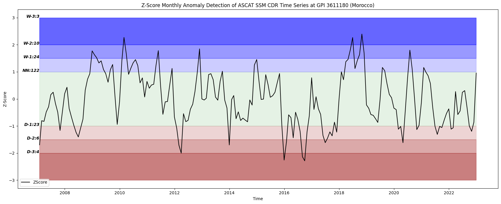
colm = {"zscore": {"color": "black", "linewidth": 1.5, "label": "ZScore"}}
plot_anomaly(
    zscore_df,
    zscore_df.index,
    colmns=colm,
    thresholds="zscore",  # For each method thresholds, refer to the source code: smadi.metadata
    plot_hbars=True,
    plot_categories=True,  # Whether to plot the number of anomalies detected in each category
    figsize=(17, 7),
    grid=False,
    legend=True,
    xlabel="Time",
    ylabel="Z-Score",
    title=f"Z-Score Monthly Anomaly Detection of ASCAT SSM CDR Time Series at GPI {gpid} (Morocco)",
)

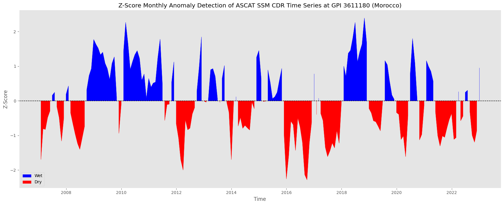
../_images/examples_detect_the_anomalies_6_0.png

[4]:

plot_fill_bet(
    zscore_df,
    zscore_df.index,
    colmn="zscore",  # Column to plot
    figsize=(17, 7),
    grid=False,
    legend=True,
    xlabel="Time",
    ylabel="Z-Score",
    title=f"Z-Score Monthly Anomaly Detection of ASCAT SSM CDR Time Series at GPI {gpid} (Morocco)",
)

../_images/examples_detect_the_anomalies_7_0.png

5.3 SMAPI Usage Example

[5]:

smapi_detector = AnomalyDetectorFactory.create_detector(
    "smapi",
    df=ascat_ts,
    variable="sm",
    fillna=True,
    fillna_window_size=3,
    smoothing=True,
    smooth_window_size=31,
    time_step="month",
    normal_metrics=["mean", "median"],
)

smapi_df = smapi_detector.detect_anomaly()
smapi_df['smapi-mean'] = smapi_df['smapi-mean'].clip(lower = -50 , upper=50)
smapi_df

[5]:

	sm-mean	norm-mean	norm-median	smapi-mean	smapi-median
2007-01-31	32.86	56.12	55.68	-41.44	-40.98
2007-02-28	36.60	47.10	47.13	-22.29	-22.35
2007-03-31	27.14	36.68	34.54	-26.00	-21.41
2007-04-30	28.36	33.51	28.39	-15.36	-0.08
2007-05-31	24.64	28.28	23.65	-12.88	4.21
...	...	...	...	...	...
2022-08-31	16.84	18.03	17.50	-6.59	-3.78
2022-09-30	17.80	21.79	22.43	-18.33	-20.67
2022-10-31	22.79	31.37	31.59	-27.33	-27.85
2022-11-30	39.96	49.91	45.05	-19.94	-11.31
2022-12-31	70.23	60.36	59.80	16.34	17.44

192 rows × 5 columns

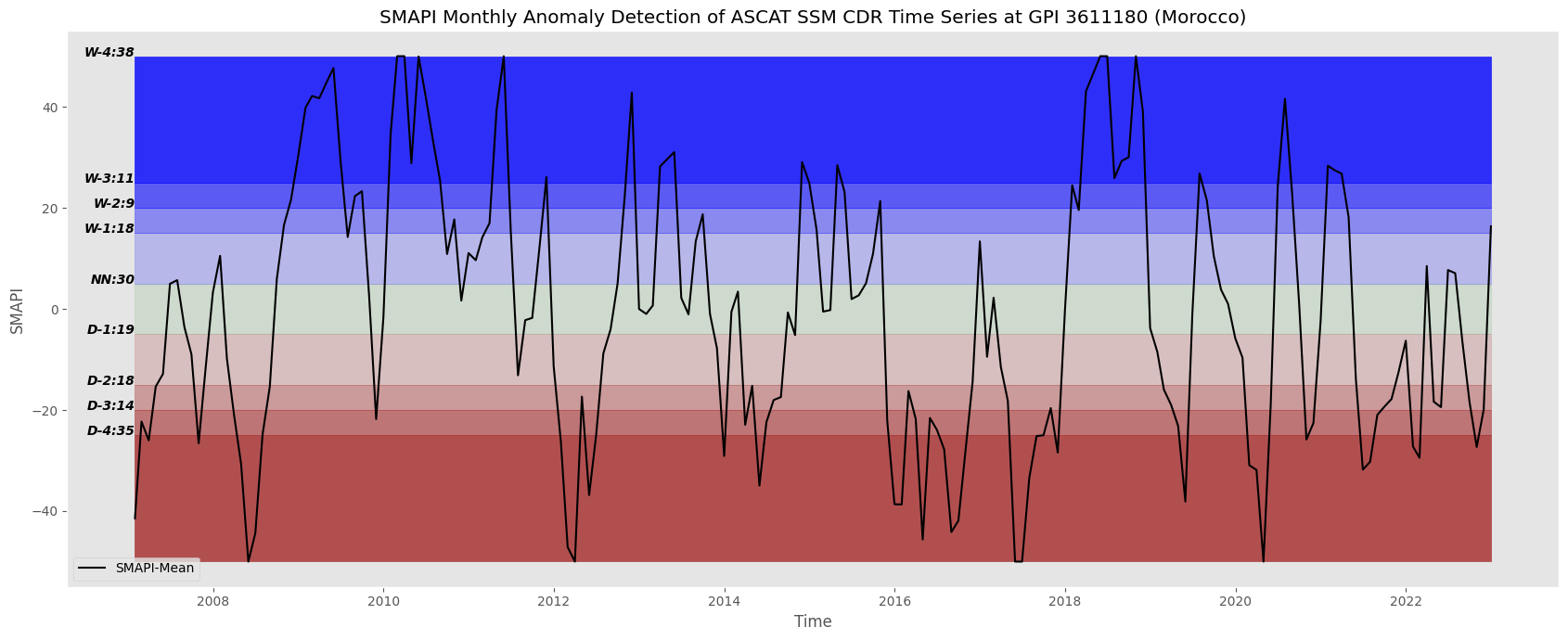
[6]:

colm = {"smapi-mean": {"color": "black", "linewidth": 1.5, "label": "SMAPI-Mean"}}


plot_anomaly(
    smapi_df,
    smapi_df.index,
    colmns=colm,
    thresholds="smapi",  # For each method thresholds, refer to the source code: smadi.metadata
    plot_hbars=True,
    plot_categories=True,  # Whether to plot the number of anomalies detected in each category
    figsize=(17, 7),
    grid=False,
    legend=True,
    xlabel="Time",
    ylabel="SMAPI",
    title=f"SMAPI Monthly Anomaly Detection of ASCAT SSM CDR Time Series at GPI {gpid} (Morocco)",
)

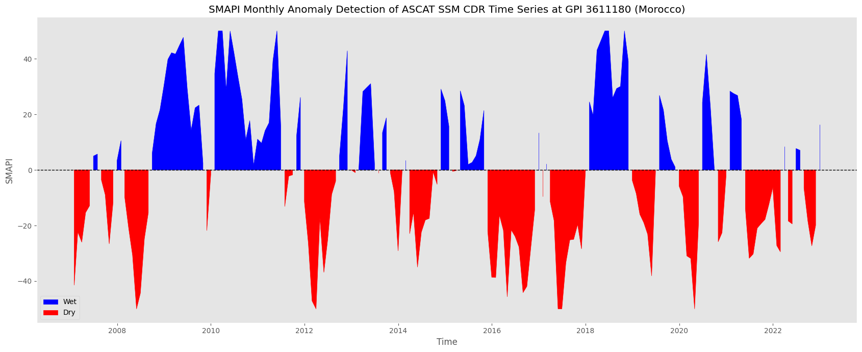
../_images/examples_detect_the_anomalies_10_0.png

[7]:

plot_fill_bet(
    smapi_df,
    smapi_df.index,
    colmn="smapi-mean",  # Column to plot
    figsize=(17, 7),
    grid=False,
    legend=True,
    xlabel="Time",
    ylabel="SMAPI",
    title=f"SMAPI Monthly Anomaly Detection of ASCAT SSM CDR Time Series at GPI {gpid} (Morocco)",
)

../_images/examples_detect_the_anomalies_11_0.png

5.4 ParaDis Usage Example

[10]:

paradis_detector = AnomalyDetectorFactory.create_detector(
    "paradis",
    df=ascat_ts,
    variable="sm",
    fillna=True,
    fillna_window_size=3,
    smoothing=True,
    smooth_window_size=31,
    time_step="month",
    dist=["beta", "gamma"],
)

para_dist_df = paradis_detector.detect_anomaly()
para_dist_df

[10]:

	sm-mean	norm-mean	beta	gamma
2007-01-31	32.86	56.12	-3.00	-1.72
2007-02-28	36.60	47.10	-0.31	-0.77
2007-03-31	27.14	36.68	-0.49	-0.83
2007-04-30	28.36	33.51	-0.26	-0.47
2007-05-31	24.64	28.28	-0.60	0.03
...	...	...	...	...
2022-08-31	16.84	18.03	-0.71	-0.30
2022-09-30	17.80	21.79	-0.52	-0.97
2022-10-31	22.79	31.37	-1.70	-1.65
2022-11-30	39.96	49.91	-0.38	-0.56
2022-12-31	70.23	60.36	0.62	0.94

192 rows × 4 columns

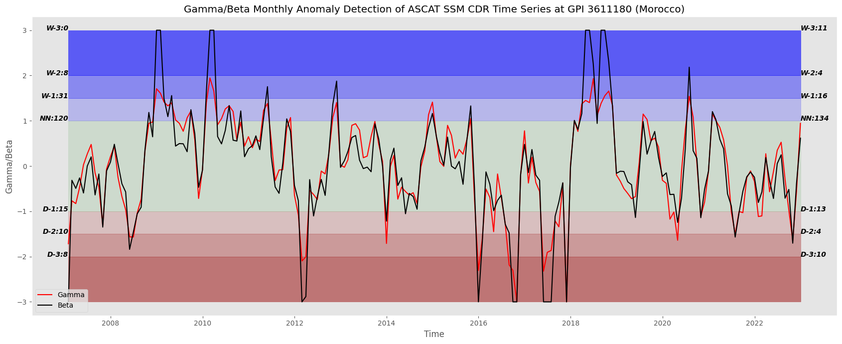
[11]:

colm = {
    "gamma": {"color": "red", "linewidth": 1.5, "label": "Gamma"},
    "beta": {"color": "black", "linewidth": 1.5, "label": "Beta"},
}

plot_anomaly(
    para_dist_df,
    para_dist_df.index,
    colmns=colm,
    thresholds="gamma",  # For each method thresholds, refer to the source code: smadi.metadata
    plot_hbars=True,
    plot_categories=True,  # Whether to plot the number of anomalies detected in each category
    figsize=(17, 7),
    grid=False,
    legend=True,
    xlabel="Time",
    ylabel="Gamma/Beta",
    title=f"Gamma/Beta Monthly Anomaly Detection of ASCAT SSM CDR Time Series at GPI {gpid} (Morocco)",
)

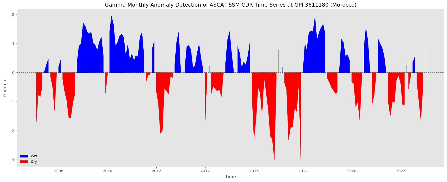
../_images/examples_detect_the_anomalies_14_0.png

[12]:

plot_fill_bet(
    para_dist_df,
    para_dist_df.index,
    colmn="gamma",  # Column to plot
    figsize=(17, 7),
    grid=False,
    legend=True,
    xlabel="Time",
    ylabel="Gamma",
    title=f"Gamma Monthly Anomaly Detection of ASCAT SSM CDR Time Series at GPI {gpid} (Morocco)",
)

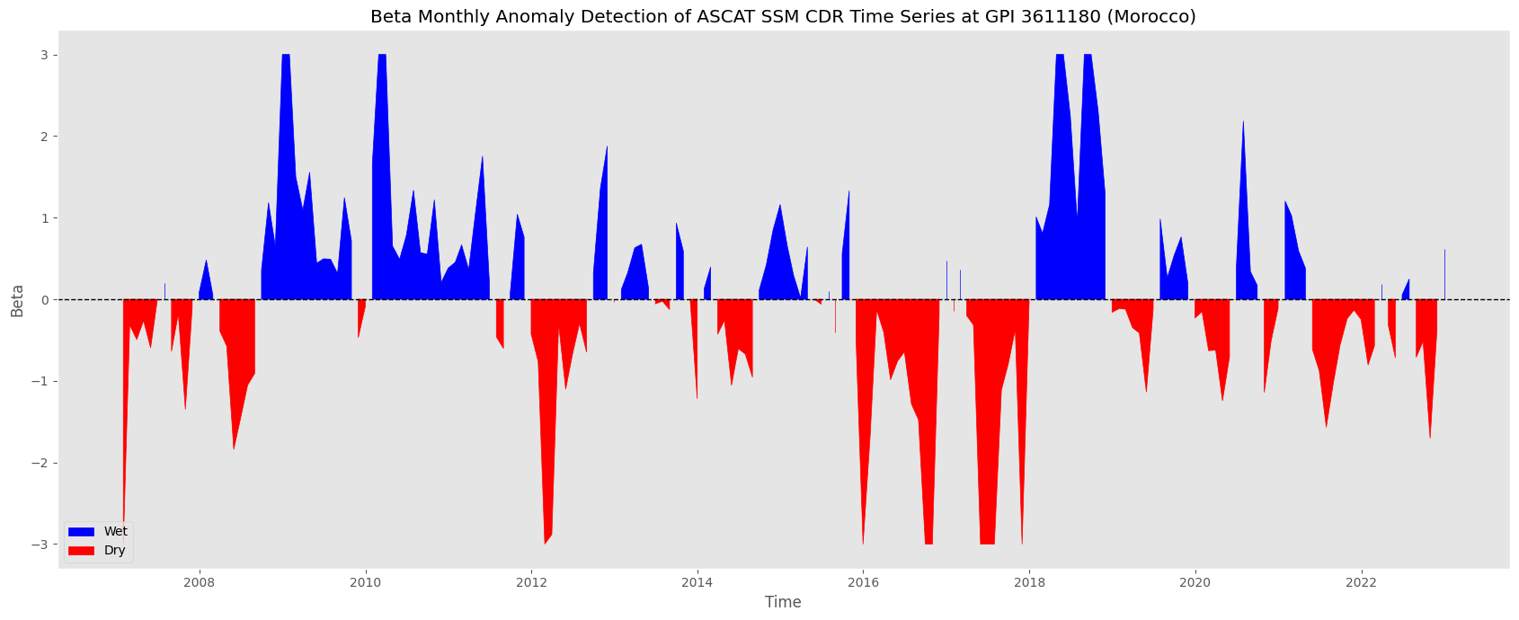
../_images/examples_detect_the_anomalies_15_0.png

[13]:

plot_fill_bet(
    para_dist_df,
    para_dist_df.index,
    colmn="beta",  # Column to plot
    figsize=(17, 7),
    grid=False,
    legend=True,
    xlabel="Time",
    ylabel="Beta",
    title=f"Beta Monthly Anomaly Detection of ASCAT SSM CDR Time Series at GPI {gpid} (Morocco)",
)

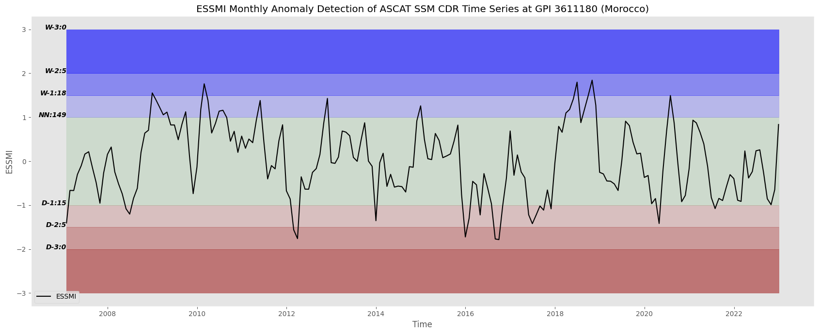
../_images/examples_detect_the_anomalies_16_0.png

5.5 ESSMI Usage Example

[14]:

essmi_detector = AnomalyDetectorFactory.create_detector(
    "essmi",
    df=ascat_ts,
    variable="sm",
    fillna=True,
    fillna_window_size=3,
    smoothing=True,
    smooth_window_size=31,
    time_step="month",
)

essmi_df = essmi_detector.detect_anomaly()
essmi_df

[14]:

	sm-mean	norm-mean	essmi
2007-01-31	32.86	56.12	-1.40
2007-02-28	36.60	47.10	-0.66
2007-03-31	27.14	36.68	-0.67
2007-04-30	28.36	33.51	-0.30
2007-05-31	24.64	28.28	-0.10
...	...	...	...
2022-08-31	16.84	18.03	-0.26
2022-09-30	17.80	21.79	-0.85
2022-10-31	22.79	31.37	-0.99
2022-11-30	39.96	49.91	-0.65
2022-12-31	70.23	60.36	0.84

192 rows × 3 columns

[15]:

colm = {"essmi": {"color": "black", "linewidth": 1.5, "label": "ESSMI"},
        }

plot_anomaly(
    essmi_df,
    essmi_df.index,
    colmns=colm,
    thresholds="essmi", # For each method thresholds, refer to the source code: smadi.metadata
    plot_hbars=True,
    plot_categories=True, # Whether to plot the number of anomalies detected in each category
    figsize=(17, 7),
    grid=False,
    legend=True,
    xlabel="Time",
    ylabel="ESSMI",
    title=f"ESSMI Monthly Anomaly Detection of ASCAT SSM CDR Time Series at GPI {gpid} (Morocco)",
)

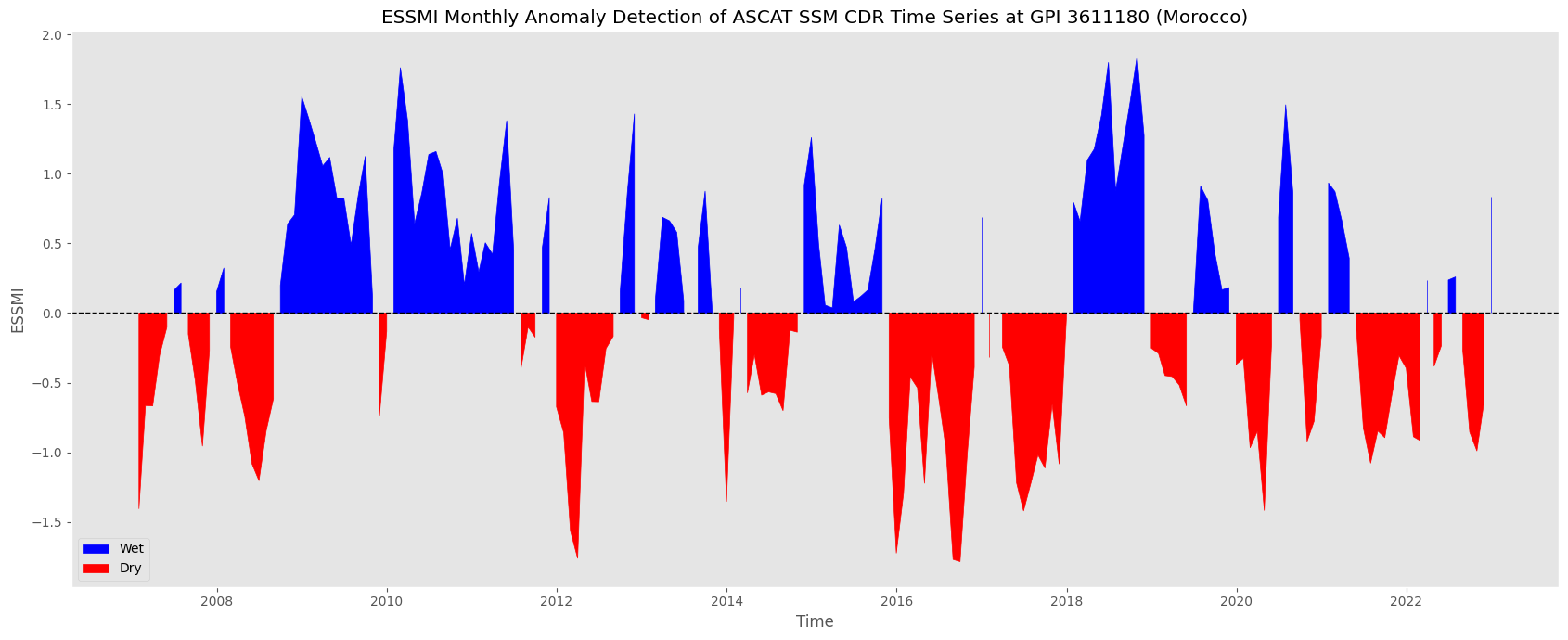
../_images/examples_detect_the_anomalies_19_0.png

[16]:

plot_fill_bet(
    essmi_df,
    essmi_df.index,
    colmn="essmi",  # Column to plot
    figsize=(17, 7),
    grid=False,
    legend=True,
    xlabel="Time",
    ylabel="ESSMI",
    title=f"ESSMI Monthly Anomaly Detection of ASCAT SSM CDR Time Series at GPI {gpid} (Morocco)",
)

../_images/examples_detect_the_anomalies_20_0.png