4. Plot the Climatology
4.1 Loading the data
[9]:
import pandas as pd
import matplotlib.pyplot as plt

from smadi.climatology import Climatology
from smadi.data_reader import read_grid_point
from smadi.plot import plot_ts

plt.style.use("ggplot")
# Set display options
pd.set_option("display.max_columns", 8)  # Limit the number of columns displayed
pd.set_option("display.precision", 2)  # Set precision to 2 decimal places

# Define the path to the ASCAT data
data_path = "/home/m294/ascat_dataset"

# Example: A grid point in Morocco
lon = -7.382
lat = 33.348
gpid = 3611180

# Define the location of the observation point
loc = (lon, lat)

# Extract ASCAT soil moisture time series for the given location
data = read_grid_point(
    loc=loc, ascat_sm_path=data_path, read_bulk=False, era5_land_path=None
)  # Provide the path to the ERA5-Land data if you want mask snow
# and frozen soil conditions. For more information about
# the dataset see ERA5-Land data documentation and to download
# use the CDS API or https://ecmwf-models.readthedocs.io/en/latest/

# Get the ASCAT soil moisture time series
ascat_ts = data.get("ascat_ts")


# Display the first few rows of the time series data
ascat_ts.head()
Reading ASCAT soil moisture: /home/m294/ascat_dataset
ASCAT GPI: 3611180 - distance:   23.713 m
Warning: ERA5-Land not found: None
Warning: ERA5 Land not found - ASCAT soil moisture not masked!
[9]:
| sm | sm_noise | as_des_pass | ssf | ... | sigma40 | sigma40_noise | num_sigma | sm_valid | |
|---|---|---|---|---|---|---|---|---|---|
| 2007-01-01 21:02:04.161 | 34.86 | 3.24 | 0 | 0 | ... | -12.27 | 0.19 | 3 | True |
| 2007-01-02 11:03:22.807 | 23.16 | 3.27 | 1 | 0 | ... | -13.05 | 0.19 | 3 | True |
| 2007-01-03 10:42:47.739 | 33.05 | 3.23 | 1 | 0 | ... | -12.39 | 0.19 | 3 | True |
| 2007-01-03 22:00:39.007 | 25.60 | 3.24 | 0 | 0 | ... | -12.88 | 0.19 | 3 | True |
| 2007-01-05 10:01:27.519 | 28.73 | 3.24 | 1 | 0 | ... | -12.67 | 0.19 | 3 | True |
5 rows × 16 columns
4.2 Plot the time series data
[11]:
# Initialize Climatology object
clim = Climatology(
    df=ascat_ts,
    variable="sm",
    time_step="week",
    fillna=True,
    fillna_window_size=3,
    smoothing=True,
    smooth_window_size=31,
    normal_metrics=["mean", "median", "min", "max", "std"],
)

# Compute normals
clim_df = clim.compute_normals()
clim_df
[11]:
| sm-mean | norm-mean | norm-median | norm-min | norm-max | norm-std | |
|---|---|---|---|---|---|---|
| 2007-01-01 | 33.29 | 56.55 | 51.97 | 33.29 | 75.79 | 13.60 |
| 2007-01-08 | 30.54 | 55.98 | 52.82 | 30.54 | 77.77 | 14.58 |
| 2007-01-15 | 34.77 | 56.58 | 57.21 | 32.46 | 79.92 | 14.96 |
| 2007-01-22 | 36.23 | 55.30 | 56.97 | 28.86 | 79.00 | 15.02 |
| 2007-01-29 | 36.65 | 54.32 | 54.77 | 31.44 | 78.50 | 14.62 |
| ... | ... | ... | ... | ... | ... | ... |
| 2022-11-21 | 49.86 | 55.10 | 53.95 | 37.34 | 75.00 | 11.74 |
| 2022-11-28 | 63.00 | 58.17 | 59.25 | 36.70 | 74.45 | 11.60 |
| 2022-12-05 | 69.93 | 61.46 | 61.16 | 36.71 | 78.51 | 12.32 |
| 2022-12-12 | 73.97 | 61.43 | 59.37 | 35.26 | 83.27 | 12.69 |
| 2022-12-19 | 72.94 | 58.85 | 58.43 | 34.96 | 78.19 | 11.38 |
838 rows × 6 columns
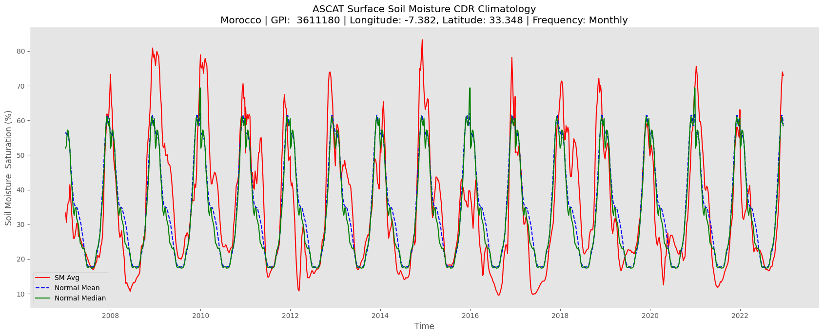
[12]:
# Set the plot options for each column
colms = {
    "sm-mean": {"color": "red", "linestyle": "-", "linewidth": 1.5, "label": "SM Avg"},
    "norm-mean": {
        "color": "blue",
        "linestyle": "--",
        "linewidth": 1.5,
        "label": "Normal Mean",
    },
    "norm-median": {"color": "green", "linewidth": 1.5, "label": "Normal Median"},
}

plot_ts(
    clim_df,
    clim_df.index,
    colmns_kwargs=colms,
    title=f"ASCAT Surface Soil Moisture CDR Climatology\nMorocco | GPI:  {gpid} | Longitude: {lon}, Latitude: {lat} | Frequency: Monthly",
    figsize=(17, 7),
    xlabel="Time",
    ylabel="Soil Moisture  Saturation (%)",
    legend=True,
    grid=False,
)
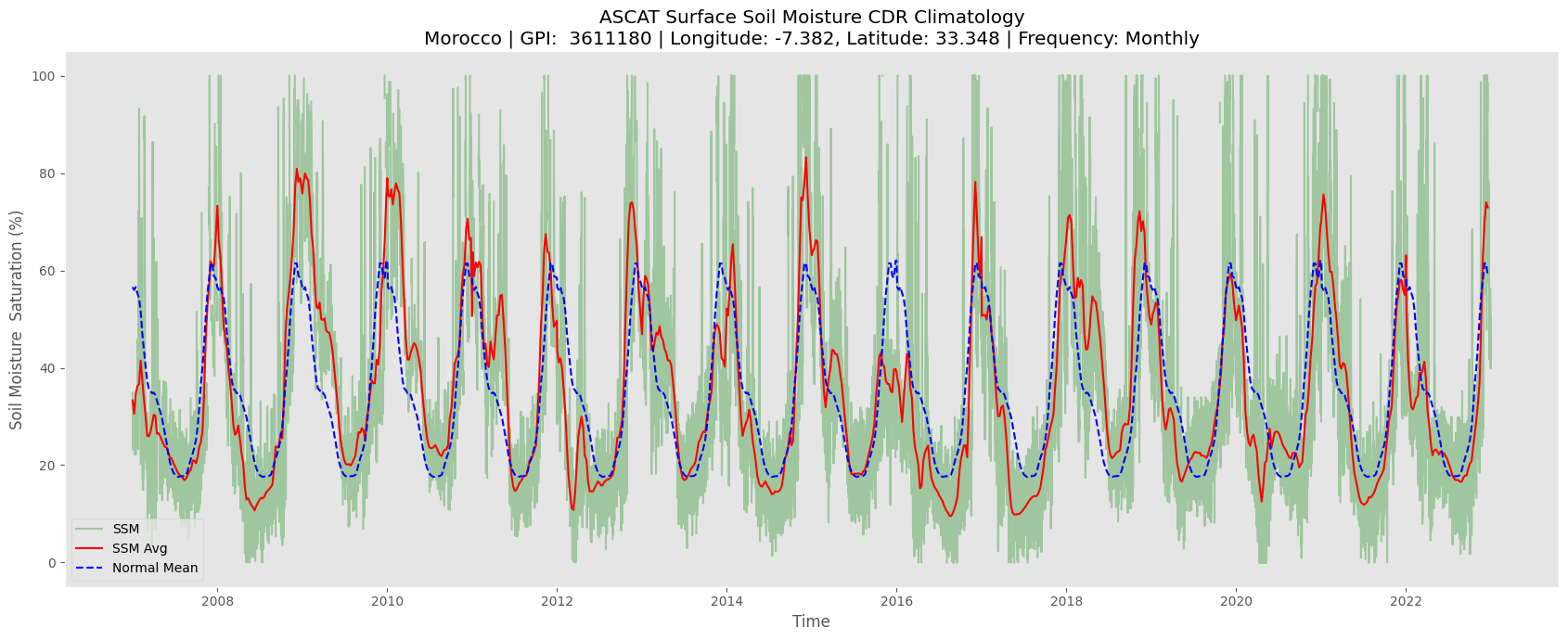
[13]:
# Set the plot options for each metric
colms = {
    "sm-mean": {"color": "red", "linestyle": "-", "linewidth": 1.5, "label": "SSM Avg"},
    "norm-mean": {
        "color": "blue",
        "linestyle": "--",
        "linewidth": 1.5,
        "label": "Normal Mean",
    },
}

# To plot the raw data, set plot_raw=True and provide the raw_kwargs for customization
plot_ts(
    clim_df,
    clim_df.index,
    colmns_kwargs=colms,
    title=f"ASCAT Surface Soil Moisture CDR Climatology\nMorocco | GPI:  {gpid} | Longitude: {lon}, Latitude: {lat} | Frequency: Monthly",
    figsize=(17, 7),
    xlabel="Time",
    ylabel="Soil Moisture  Saturation (%)",
    plot_raw=True,
    raw_df= ascat_ts,
    raw_var="sm",
    raw_kwargs={"color": "green",  "label": "SSM", "alpha": 0.3},
    legend=True,
    grid=False,
)